Capstone Project
The following is a case study I completed to apply skills like data cleaning, data processing, and data visualization that I learned from taking the Google Data Analytics Professional Course.
I had three options: selecting one of two prompts or creating my own adventure with a dataset of my choosing. For my first major project, I chose the Bellabeat prompt and utilized the R programming language for data cleaning and analysis. I learned so much!
By the way, Bellabeat is a real fitness company and their products are pretty sleek as far as fitness trackers go.
I have been asked (fictionally!) to focus on one of Bellabeat’s products and analyze smart device data to gain insight into how consumers are using their smart devices. The insights I discover will then help guide marketing strategy for the company. I will present my analysis to the Bellabeat executive team along with my high-level recommendations for Bellabeat’s marketing strategy.
This part is where a fictional senior leader, Sršen, asks me to analyze smart device usage data in order to gain insight into how consumers use non-Bellabeat smart devices. She then wants me to select one Bellabeat product to apply these insights to in your presentation. These questions will guide my analysis:
- 1. What are some trends in smart device usage?
- 2. How could these trends apply to Bellabeat customers?
- 3. How could these trends help influence Bellabeat marketing strategy?
Business Task
Identify new growth opportunities for Bellabeat’s Leaf product to inform marketing strategy by identifying trends in how consumers use their (non-Bellabeat) smart devices.
Data Sources
TL;DR
In this part I describe the data, assess if it's quality, trustworthy, where it came from, where it lives, etc. Google uses the "Does the Data ROCC?" question to help guide and assess it. Overall the dataset is full of holes. If I were actually using this data, I'd have so many questions for the stakeholders about the project and data integrity. I would most definitely want more data than contained in the datasets! Read below to get the nitty gritty, picky observations I had.
Dataset and Licensing
FitBit Fitness Tracker Data (CC0: Public Domain, dataset made available through Mobius). It’s open source and the data is updated annually. The last update was 8 months ago.
→ FitBit Fitness Tracker DataData Collection
This Kaggle data set contains personal fitness tracker data from 35 Fitbit users over a two-month period between 03.12.2016-05.12.2016. Thirty-five eligible Fitbit users consented to the submission of quantitative personal tracker data, including minute-level output for physical activity, heart rate, and sleep monitoring. It includes information about daily activity, steps, and heart rate that can be used to explore users’ habits.
Data Organization (filtering and sorting)
The dataset contains primary, structured data in 29 CSV files; 11 CSV files are for the first month of data from 3.12.16 - 4.11.16 and the other 18 CSV files are for the second month of data from 4.12.16 - 5.12.16. The dataset is in long format with multiple entries per user Id. I used Google Sheets to preview an inspect the datasets.
Does this data ROCCC?
Reliable
It’s inconclusive whether the sample size represents the overall population, though the 35-user size meets the minimum Central Limit Theorem (CLT) requirements for validity. Much of the data is incomplete for each user and not all data sets contain data for each of the 35 users. Using a sample size calculator from SurveyMonkey would help determine the ideal sample size that would accurately reflect the greater population of users who use smart devices. Additionally, the metadata on the datasets lacks details about the confidence level and margin of error for the sample population.
Other Considerations
- The timeframe for data collection was limited to 2 months, which may give a limited view of the device usage. This could be a problem since device usage may vary with seasonality and user adoption of a new technology or tool.
- Calories doesn't indicate if it's calories burned or calories consumed. For the purpose of this study, we'll assume it's calories burned.
- The data points are reliable as they were tracked and recorded by the devices.
- The data does not specify the units of measurement for most variables involving distance or intensity. For example, we cannot determine whether distance is measured in miles, kilometers, feet, or another unit. Additionally, the method used to assess and categorize activity levels—ranging from sedentary to very active or moderately active—remains unclear.
- It is unclear whether the distance recorded in "logged activities" is a manual input or a feature of the FitBit device.
Original
The data is an original data source.
Comprehensive
The sample size is small and lacks essential demographic information, which is crucial for addressing the business task. For instance, gender is particularly important for Bellabeat products, as they are marketed specifically to women. Ideally, the dataset should include gender information to help Bellabeat identify trends among smart device users based on gender. Additionally, the FitBit dataset does not specify the type of fitness tracker from which the data originates—whether it is a wearable device, an app, etc. This report will provide a preliminary analysis.
Current
This data is nearly a decade old. Since it was collected, technology and fitness trackers have evolved significantly, so making recommendations for 2024 based on old data may lead to poor outcomes, though it could be interesting to compare this study with data from more recent years to determine if these same trends still exist today.
Cited
The source was cited and vetted.
Privacy, Security, and Accessibility
The original dataset is stored in this folder in GDrive. Stakeholders have permission to view the dataset.
The cleaned dataset is stored in this folder in GDrive. Stakeholders have permission to view and comment on the dataset.
Documentation Cleaning or Manipulation of Data
Renaming Datasets
I renamed each dataset I will use to reflect the timeframe it represents, allowing for easier merging in R. The datasets I will be using for this Case Study are as follows:
Installing Packages in R
I installed the following packages to clean and analyze the data.
{R}
install.packages(c("tidyverse", "skimr", "janitor", "lubridate", "here", "outliers"))
- library (tidyverse)
- library (skimr)
- library (janitor)
- library (lubridate)
From here, I realized that trying to clean and combine hourly data and daily data would be a mess in one script. I chose to split datasets into two different {R} Scripts for ease of analysis. The first set of scripts is for Hourly Activity. The second set of scripts is for Daily Activity.
Hourly Activity Datasets
Uploading and Combining Datasets
There are six total datasets for hourly activity that need to be combined. The final merge combined all of the data by Id and ActivityHour columns.
 {R}

                hourly_intensities_1 <- read_csv("hourlyIntensities_3.12.16-4.11.16.csv") head(hourly_intensities_1) colnames(hourly_intensities_1)

                    hourly_intensities_2 <- read_csv("hourlyIntensities_4.12.16-5.12.16.csv") head(hourly_intensities_2) colnames(hourly_intensities_2)

                        hourly_intensity <- rbind(hourly_intensities_1, hourly_intensities_2) glimpse(hourly_intensity)
{R}

                hourly_steps_1 <- read_csv("hourlySteps_3.12.16-4.11.16.csv") head(hourly_steps_1) colnames(hourly_steps_1)

                    hourly_steps_2 <- read_csv("hourlySteps_4.12.16-5.12.16.csv") head(hourly_steps_2) colnames(hourly_steps_2)

                        hourly_steps <- rbind(hourly_steps_1, hourly_steps_2) glimpse(hourly_steps)
{R}

                 hourly_calories_1 <- read_csv("hourlyCalories_3.12.16-4.11.16.csv") head(hourly_calories_1) colnames(hourly_calories_1)

                    hourly_calories_2 <- read_csv("hourlyCalories_4.12.16-5.12.16.csv") head(hourly_calories_2) colnames(hourly_calories_2)

                        hourly_calories <- rbind(hourly_calories_1, hourly_calories_2) glimpse(hourly_calories)
{R}
 hourly_activity_df <- merge(hourly_intensity, hourly_steps, by=c ("Id", "ActivityHour" )) glimpse(hourly_activity_df)
The {R} script below shows the result from the final merge above with hourly_calories by Id and ActivityHour into one final dataframe, hourly_activity_final. This dataframe contains all of the hourly activity from all six imported files!
Perhaps there is a more efficient way to do this?
{R}
hourly_activity_final <- merge(hourly_activity_df, hourly_calories, by=c("Id", "ActivityHour" )) glimpse(hourly_activity_final) str(hourly_activity_final) summary(hourly_activity_final)
Viewing Structure and Summarizing Data
I peformed the follwing functions to check that the data was combined and merged properly.
- Viewed the structure with str() to know what data types are in each column.
- Use summary() to get an overview of the data sets.
- Used glimpse() to preview data.
Console
 > summary(hourly_activity_final)

            Id ActivityHour TotalIntensity AverageIntensity StepTotal
            Min. :1.504e+09 Length:47233 Min. : 0.0 Min. :0.00000 Min. : 0.0
            1st Qu.:2.320e+09 Class :character 1st Qu.: 0.0 1st Qu.:0.00000 1st Qu.: 0.0
            Median :4.559e+09 Mode :character Median : 2.0 Median :0.03333 Median : 17.0
            Mean :4.868e+09 Mean : 11.3 Mean :0.18836 Mean : 300.1
            3rd Qu.:6.962e+09 3rd Qu.: 15.0 3rd Qu.:0.25000 3rd Qu.: 317.0
            Max. :8.878e+09 Max. :180.0 Max. :3.00000 Max. :10565.0
            Calories
            Min. : 42.00
            1st Qu.: 62.00
            Median : 80.00
            Mean : 95.43
            3rd Qu.:105.00
            Max. :948.00
Removing Duplicates and Trimming Whitespace
First I trimmed the whitespace, then I checked for duplicates. There were 35 user Ids and 1225 duplicates found. I then removed the duplicates.
 {R}

                #trimming leading/trailing spaces
                 hourly_activity_final <-hourly_activity_final %>%
                    mutate(across(everything(), trimws))
                #Check for duplicates
                n_unique(hourly_activity_final$Id) #35 unique Ids

                sum(duplicated(hourly_activity_final)) #1225 duplicates found

                #Remove duplicates based on Id, keeping all other columns
                 hourly_activity_final <- hourly_activity_final %>%
                    distinct() %>%
                    drop_na()
                sum(duplicated(hourly_activity_final))
Cleaning Column Names
{R}

                #cleaning column names
                 hourly_activity_final<- hourly_activity_final %>% #cleaning column names
                    clean_names()
                head(hourly_activity_final)
                colnames(hourly_activity_final)
Converting Data Types in Columns
Here I convert data types into numbers to make calculations based on time of day.
{R}

                hourly_activity_final$average_intensity <-as.numeric(hourly_activity_final$average_intensity)< /p>
                    #convert 'average_intensity' column to number
                    hourly_activity_final$total_intensity <-as.numeric(hourly_activity_final$total_intensity)< /p>
                         #convert 'total_intensity' column to number
                        hourly_activity_final$step_total <-as.numeric(hourly_activity_final$step_total)< /p>
                             #convert 'step_total' column to number
                            hourly_activity_final$calories <-as.numeric(hourly_activity_final$calories)< /p>
                                 #convert 'calories' column to number
                                glimpse(hourly_activity_final)
Here I convert the time column to make calculations based on time of day. I chose to translate each hour into a two digit number IE 13:00 = 13.
{R}

                 hourly_activity_final_cleaned <- hourly_activity_final %>%
                    mutate(hour = substr(time, 1, 2)) # Extract first two characters from 'time' column

                hourly_activity_final_cleaned$hour <-as.numeric(hourly_activity_final_cleaned$hour)< /p>
                    #convert 'hour' column to number

                    print(hourly_activity_final_cleaned) # Print the data frame to check the result
Hiding Columns
Hiding the activity-hour column (it was a date-time column) to reduce visual clutter in the data frame.
{R}

                hourly_activity_final_cleaned <- hourly_activity_final_cleaned %>% select(-activity_hour)

                glimpse(hourly_activity_final_cleaned)
                head(hourly_activity_final_cleaned)
Daily Activity Datasets
Uploading and Combining Datasets
There are two total datasets for daily activity that need to be uploaded and combined.
 {R}

                #Importing daily activity datasets.
                daily_activity_1 <- read_csv("dailyActivity_3.12.16-4.11.16.csv") head(daily_activity_1) colnames(daily_activity_1)

                    daily_activity_2 <- read_csv("dailyActivity_4.12.16-5.12.16.csv") head(daily_activity_2) colnames(daily_activity_2)

                        #Combining the two data sets for daily activity. Renamed to daily_activity.
                        daily_activity <- rbind(daily_activity_1, daily_activity_2) glimpse(daily_activity) str(daily_activity) summary(daily_activity)
Removing Duplicates and Trimming Whitespace
First I trimmed the whitespace, then I checked for duplicates. No duplicates found!
Daily {R}

                #trimming leading/trailing spaces
                daily_activity <-daily_activity %>%
                    mutate(across(everything(), trimws))

                #removing duplicates
                n_unique(daily_activity$Id)
                  sum(duplicated(daily_activity)) #no duplicates found!
Cleaning Column Names and Hiding Columns
I hid the unnecessary columns "logged activities"logged_activities_distance" and "tracker_distance" to reduce clutter in the dataframes.
 {R}

                #formatting and cleaning column names
                daily_activity <- daily_activity %>%
                    clean_names()
                    head(daily_activity)
                    colnames(daily_activity)

                #hiding unnecessary columns "logged activities"logged_activities_distance" and "tracker_distance"
                daily_activity <- daily_activity %>% select(-logged_activities_distance, -tracker_distance)
Converting Datatypes in Columns
I changed the date column into a date format from a character format and changed most of the other columns to numbers, with the excecption of id.
 {R}

                daily_activity$activity_date <- as.Date(daily_activity$activity_date, format="%m/%d/%Y" ) #Changed it from a character data type to a date.

                    daily_activity <- daily_activity %>%
                        mutate(across(c(
                        total_steps,
                        total_distance,
                        very_active_distance,
                        moderately_active_distance,
                        light_active_distance,
                        sedentary_active_distance,
                        very_active_minutes,
                        fairly_active_minutes,
                        lightly_active_minutes,
                        sedentary_minutes,
                        calories),
                        as.numeric))

                    str(daily_activity) #checking that the new formatting worked!
Creating New Columns
I created new columns: "day_type" to label each day as a weekday or weekend, "day_of_week" to label each day of the week, and "week_number" to number each week from 1-9.
 {R}

                #creating new columns for weekdays and weekends
                daily_activity_cleaned <- daily_activity %>%
                    mutate(day_type = ifelse(wday(activity_date) %in% c(1, 7), "Weekend", "Weekday"))

                #creating new column to label each day by the day of the week.
                daily_activity_cleaned$day_of_week <- wday(daily_activity_cleaned$activity_date, label=TRUE, abbr=FALSE) glimpse(daily_activity_cleaned)
                #creating new column to label each week of the data collected (1 -8)
                #date range
                start_date <- ymd("2016-03-12") end_date <- ymd("2016-05-12")
                    #sequence of dates
                    date_range <- seq.Date(start_date, end_date, by="day" )

                        #week number
                        daily_activity_cleaned$week_number <- ceiling(as.numeric(difftime(daily_activity_cleaned$activity_date, start_date, units="days" ) + 1 )/ 7)

                            glimpse(daily_activity_cleaned) #checking that the new formatting worked!
Hourly Activity Analysis
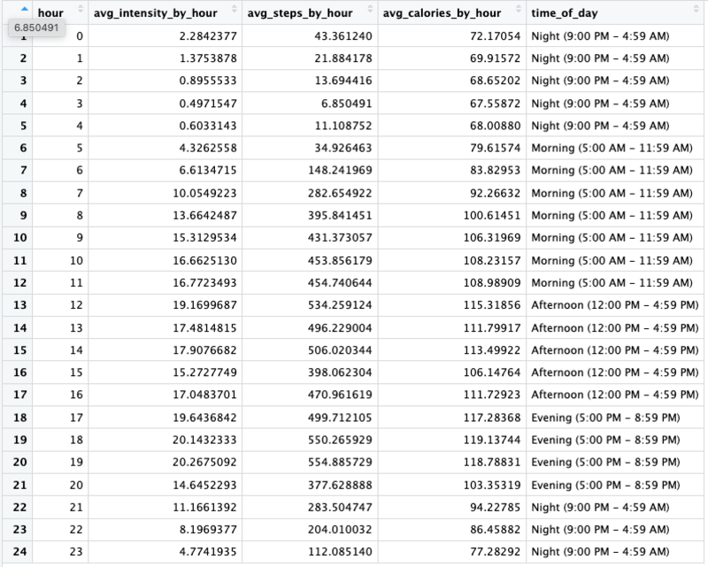
Average Intensity by Hour
Grouping by time to get all of the ids exercising at 1pm, for example, to group together with average intensity at a specific hour.
{R}

            hourly_summary <- hourly_activity_final_cleaned %>%
                group_by(hour) %>% #group by hour
                summarize(
                avg_intensity_by_hour = mean(total_intensity, na.rm = TRUE),
                avg_steps_by_hour = mean(step_total, na.rm = TRUE),
                )

            print(hourly_summary)
            glimpse(hourly_summary)
Grouping Avgerage Intensity by Time of Day
Assigned labels to ranges of hours during the day like morning, afternoon, evening, and night.
{R}

            hourly_summary <- hourly_summary %>%
                mutate(
                time_of_day = case_when(
                hour >= 5 & hour < 12 ~ "Morning (5:00 AM - 11:59 AM)" , hour>= 12 & hour < 17 ~ "Afternoon (12:00 PM - 4:59 PM)" , hour>= 17 & hour < 21 ~ "Evening (5:00 PM - 8:59 PM)" , TRUE ~ "Night (9:00 PM - 4:59 AM)" ) )
Summary of Analysis for Hourly Activity
Calculations
- Created new columns for date and time
- Assigned labels to each time of day (night, morning, afternoon, evening)
- Calculated the average intensity by hour for all users
- Calculated the average steps by hour for all users
These calculations will help us visualize and determine if there is a specific time of day and/or hour when activity is higher for users.
Daily Activity Analysis
Daily Activity Usage Summary by id
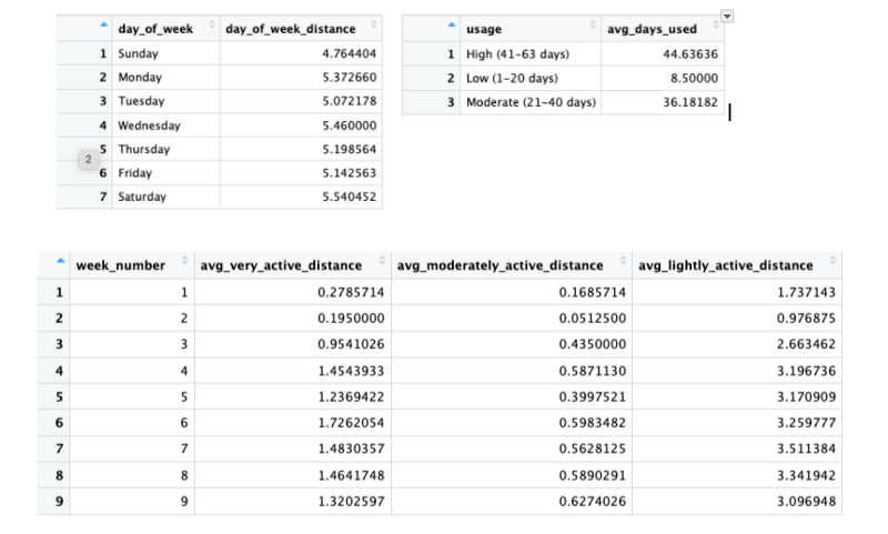
Finding the avereage days used by id from Low to High usage categories. Low usage is 1-20 days, Moderate is 21-40 days,High is 41-63 days.
{R}

            daily_usage_by_id_summary <- daily_activity_cleaned %>%

                group_by(id) %>%

                summarize(
                days_used=sum(n())) %>%

                mutate(usage = case_when(
                days_used >= 1 & days_used <= 20 ~ "Low (1-20 days)" , days_used>= 21 & days_used <= 40 ~ "Moderate (21-40 days)" , days_used>= 41 & days_used <= 64 ~ "High (41-63 days)" , ))
Grouping the Average Days Used by Usage Category
Finding the avereage days used from Low to High usage categories. Low usage is 1-20 days, Moderate is 21-40 days,High is 41-63 days.
{R}

            #finding the average days used by usage category
              daily_avg_usage_summary <- daily_usage_by_id_summary %>%
                group_by(usage) %>%
                summarize(
                avg_days_used = mean(days_used, na.rm = TRUE)
                ) %>%
                mutate(
                percentage = (avg_days_used / sum(avg_days_used)) * 100
                )

                daily_avg_usage_summary$usage <- factor(daily_avg_usage_summary$usage, levels=c( "Low (1-20 days)" , "Moderate (21-40 days)" , "High (41-63 days)" )) str(daily_avg_usage_summary) daily_activity_percent_usage_summary <- daily_avg_usage_summary %>% #avg percentage of days used during data collection period (63 days)
                  group_by(usage) %>%
                  summarize (
                  percent_used = round((avg_days_used/63) *100,0)
                  )
Summarizing Weekly Averages by Distance Type
Very Active Distance | Moderately Active Distance | Lightly Active Distance
{R}

            week_distance_type_summary <- daily_activity_cleaned %>%
                group_by(week_number) %>%

                summarize (
                avg_very_active_distance = mean(very_active_distance, na.rm = TRUE),
                avg_moderately_active_distance = mean(moderately_active_distance, na.rm = TRUE),

                avg_lightly_active_distance = mean(light_active_distance, na.rm = TRUE)
                )


                #converting data into a long format for creating a chart.
                week_distance_type_summary_long <- week_distance_type_summary %>%

                  pivot_longer(cols = starts_with("avg"),

                  names_to = "activity_level",

                  values_to = "average_distance"

                  )
Average Total Distance by Week
Finding the average distance by the week number from 1 to 9.
{R}

            week_count_distance_summary <- daily_activity_cleaned %>%
                group_by(week_number) %>%
                summarize (
                weekly_distance = mean(total_distance, na.rm = TRUE))
{R}

            weekday_distance_summary <- daily_activity_cleaned %>%
                group_by(day_of_week) %>%
                summarize (
                day_of_week_distance = mean(total_distance, na.rm = TRUE))
Summary of Analysis for Daily Activity
Calculations
- Grouped users by days used and put them in newly created categories for usage level from low to high
- Summarized the number of days used by each usage level.
- Calculated the weekly averages by distance type.
- Calculated the average total distance by the day of the week.
- Calculated the average total distance by week count.
These calculations will help us determine if (1) the average intensity of activity that most users do (2) if there is a specific day of the week or week during the data collection period when activity is higher for users which is determined by distance.
Hourly Activity Visualizations
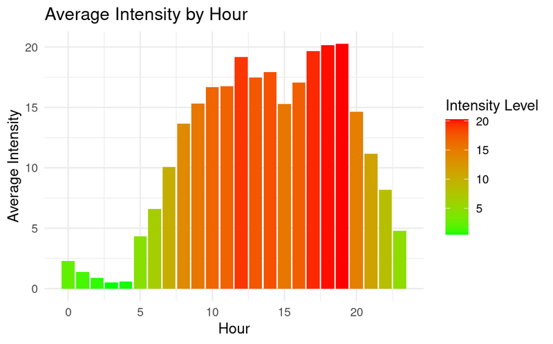
The chart above reveals that users are most active between 8am and 8pm with the highest activity hours being 12:00pm and from 5:00pm - 8:00pm.
{R}

              ggplot(hourly_summary, aes (x = hour, y = avg_intensity_by_hour, fill = avg_intensity_by_hour)) +

                geom_col() +

                scale_fill_gradient(low = "green", high = "red") +

                theme_minimal() +

                labs(title = "Average Intensity by Hour", x = "Hour", y= "Average Intensity")
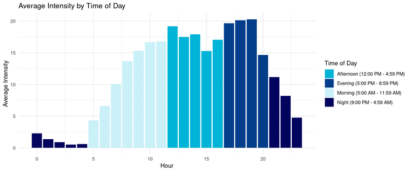
The chart above further shows that intensity is higher in the evening followed closely by the afternoon. I decided to group hours of the day by time of day, IE "morning" to help illustrate futher how activity varies by the time of the day.
{R}

                ggplot(hourly_summary, aes (x = hour, y = avg_intensity_by_hour, fill = time_of_day)) +

                  geom_col() +

                  scale_fill_manual(values= c("Morning (5:00 AM - 11:59 AM)" = "#caf0f8",
                  "Afternoon (12:00 PM - 4:59 PM)" = "#00b4d8",
                  "Evening (5:00 PM - 8:59 PM)" = "#023e8a",
                  "Night (9:00 PM - 4:59 AM)" = "#03045e")) +

                  theme_minimal() +


                  labs(title = "Average Intensity by Time of Day", y= "Average Intensity", x= "Hour", fill = "Time of Day")
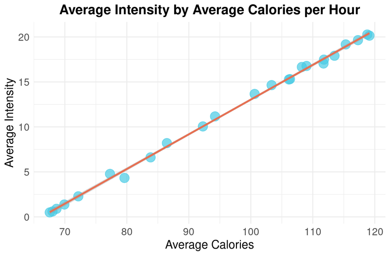
The scatterplot above shows that there is a positive correlation between intensity and calories burned in an hour. It seems obvious but confirms that with more intensity, more calories are burned.
{R}

                  ggplot(hourly_summary, aes(x=avg_calories_by_hour, y=avg_intensity_by_hour)) +

                    geom_point(color="#48cae4", size = 5, alpha = 0.7) +

                    geom_smooth(method = "lm", color = "#e76f51") + #trendline

                    labs(
                    title = "Average Intensity by Average Calories per Hour",
                    x = "Average Calories",
                    y = "Average Intensity"
                    ) + #adding labels
                    theme_minimal()+

                    theme(
                    plot.title = element_text(hjust = 0.5, size = 16, face = "bold"),
                    axis.title = element_text(size = 14),
                    axis.text = element_text(size = 12)
                    ) #adjusting sizes of labels
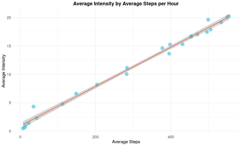
The scatterplot above shows that there is a positive correlation between intensity and steps each hour. It seems obvious but confirms that with more steps per hour, there is more intensity.
{R}

                    ggplot(hourly_summary, aes(x=avg_steps_by_hour, y=avg_intensity_by_hour)) +

                      geom_point(color="#48cae4", size = 5, alpha = 0.7) +

                      geom_smooth(method = "lm", color = "#e76f51") + #trendline

                      labs(
                      title = "Average Intensity by Average Steps per Hour",
                      x = "Average Steps",
                      y = "Average Intensity"
                      ) + #adding labels
                      theme_minimal()+

                      theme(
                      plot.title = element_text(hjust = 0.5, size = 16, face = "bold"),
                      axis.title = element_text(size = 14),
                      axis.text = element_text(size = 12)
                      ) #adjusting sizes of labels
Daily Activity Visualizations
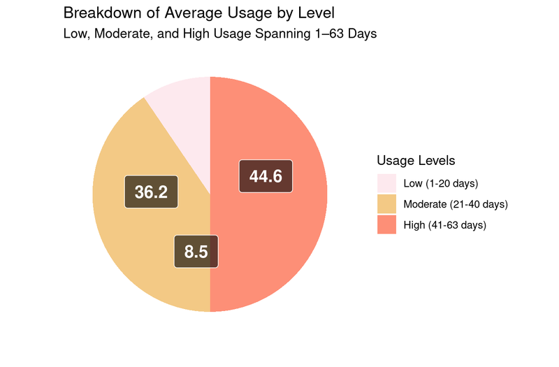
The pie chart above shows the distribution of average days used across three defined usage levels. It shows that out of the 35 unique users, about half fell into the low or moderate usage categories.
{R}

                        ggplot(daily_avg_usage_summary, aes(x= "", y =avg_days_used, fill = usage)) +

                          geom_bar(stat = "identity", width = 1) + # Use geom_bar for pie chart

                          scale_fill_manual(values = c(
                          "Low (1-20 days)" = "#fde9ee",
                          "Moderate (21-40 days)" = "#f3c985",
                          "High (41-63 days)" = "#fd8f77")) +
                          coord_polar("y", start = 0) + # Convert to polar coordinates for a pie chart

                          theme_minimal() +

                          theme(
                          axis.text.x = element_blank(), #Remove x axis text
                          axis.text.y = element_blank(), #Remove y axis text
                          axis.ticks = element_blank(), # Remove axis ticks
                          panel.grid = element_blank() # Remove grid lines
                          ) +

                          geom_label(aes(label = paste0(round(avg_days_used, 1))),  # Add percentage labels
                          position = position_stack(vjust = 0.4),  # Position the labels inside the slices
                          color = "white", size = 5, fontface = "bold",  # Text color and size
                          label.padding = unit(0.5, "lines"),  # Add padding around the text
                          fill = "black", alpha = 0.6) +

                          labs(
                          title = "Breakdown of Average Usage by Level",
                          subtitle = "Low, Moderate, and High Usage Spanning 1–63 Days",
                          fill = "Usage Levels",
                          x = "",
                          y = ""
                          )
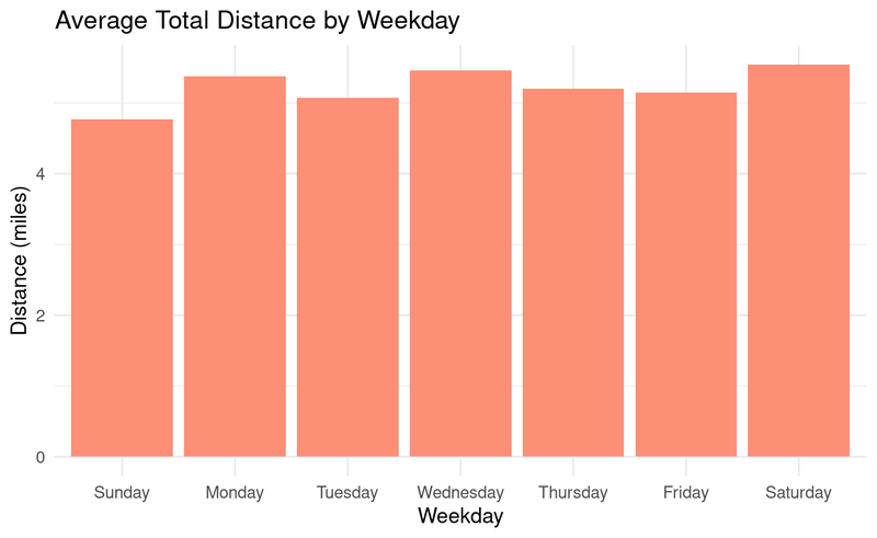
The chart above shows that Monday, Wednesday and Saturdays are the days with higher distances logged throughout the week.
{R}

                          ggplot(weekday_distance_summary, aes(x = day_of_week, y = day_of_week_distance))+

                            geom_col(fill = "#fd8f77") +

                            theme_minimal() +

                            labs(
                            title = "Average Total Distance by Weekday",
                            fill = "Weekday",
                            x = "Weekday",
                            y = "Distance (miles)"
                            )
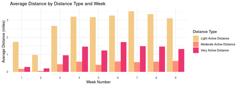
The chart above shows that over a period of 9 weeks, the most users fall into the lightly active category and less activity overall in the first three weeks.
{R}

                            ggplot(week_distance_type_summary_long, aes(x = factor(week_number), y = average_distance, fill = activity_level)) +

                              geom_bar(stat = "identity", position = "dodge") +

                              scale_fill_manual(values= c("avg_lightly_active_distance" = "#f3c985",
                              "avg_moderately_active_distance" = "#fd8f77",
                              "avg_very_active_distance" = "#ec3672"),
                              labels= c("avg_lightly_active_distance" = "Light Active Distance",
                              "avg_moderately_active_distance" = "Moderate Active Distance",
                              "avg_very_active_distance" = "Very Active Distance")) +

                              labs (
                              title = "Average Distance by Distance Type and Week",
                              x = "Week Number",
                              y = "Average Distance (miles)",
                              fill = "Distance Type") +

                              theme_minimal()
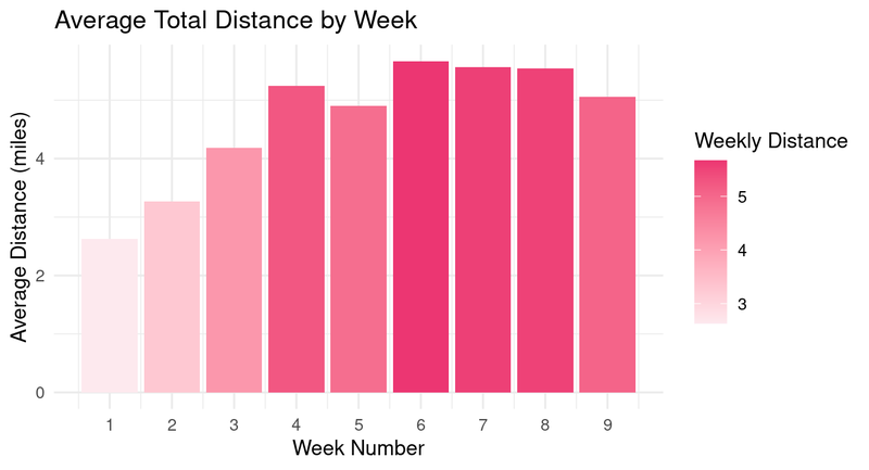
The chart above shows that over a period of 9 weeks, the first three weeks have less distance logged.
{R}


                                ggplot(week_count_distance_summary, aes(x = week_number, y = weekly_distance, fill = weekly_distance))+

                                geom_col() +

                                scale_fill_gradient(low = "#fde9ee", high = "#ec3672") +
                                theme_minimal() +

                                labs(
                                title = "Average Total Distance by Week",
                                fill = "Weekly Distance",
                                x = "Week Number",
                                y = "Average Distance (miles)"
                                ) +

                                scale_x_continuous(breaks = seq(min(week_count_distance_summary$week_number),

                                max(week_count_distance_summary$week_number), by = 1))
Top High-Level Recommendations Based on My Analysis
Fitness Onboarding and Habit Formation
The data shows a trend that in the first three weeks of usage, there is lower activity overall, this suggests that new users wore their device less during the first three weeks as they built a habit of wearing it, or they were starting a new exercise regime. I recommend creating reminders or goals for new users, as a sort of “fitness onboarding” so that new users develop a habit of wearing their devices and thereby using the device more from the start. Fitness onboarding can help users form habits, especially if they are new to wearing such devices.
I suggest features like:
Rewards for Streaks
Since roughly half of the users fall into the Low to Moderate use categories, I’d create rewards for being on a streak of using the device. Gamifying the experience with rewards for streaks is a way to enhance engagement with the device and increase usage.
I suggest rewards like:
Goal Setting for Running or Walking Events
Most users are “lightly active” based on distance, with “very active distance” being the second category. Since distance is measured by steps, I’d create goal-setting features and training plans by activity level for users training for running or walking events like marathons, 5Ks, etc. Most users being lightly active suggests that aspirational goal-setting features could motivate them to increase their activity levels.
Customizable Calorie Burning Goals
From the two scatterpolots we can see that as intensity increases, so do steps, and calories burned. I’d offer a way for users to pick their calorie-burning goal based on either intensity or steps. This will help users burn calories in a way they prefer. Giving users flexibility to align goals with their preferences (intensity vs. steps) adds personalization, which is valuable for user engagement.
I suggest features like: